Carto tips: Using blend modes and opacity levels
There are many things we can do to the features on our maps to change their appearance and many techniques we can apply to adjust the colours. Adjusting opacity levels and applying blend modes are the two techniques that we will explore in this post and we will look at some examples of how we can use them together to create effective visualisations.
So, what are blend modes?
OK, the obvious bit first. Opacity levels are on a scale from 0-100%; where 100% is fully opaque and 0% is fully transparent. Blend modes however are a little less obvious and there are many to choose from. Essentially they affect how the colours of different features interact with each other by darkening, lightening and/or blending and can also let us ‘see through’ features.
Let’s look at some of the most commonly-used options:
Multiply
This is the best mode for darkening (and to be honest it’s the one I use most often.) It multiplies the luminance levels of the current layer’s pixels with the pixels in the layers below. It is good for removing whites whilst maintaining darker colours.
Screen
This does the opposite to multiply so it multiplies the light pixels.
Overlay
Uses a combination of the Screen blend mode on the lighter pixels, and the Multiply blend mode on the darker pixels. It uses a half-strength application of these modes, and the mid-tones (50% grey) become transparent.
Addition
This blend mode simply adds pixel values of one layer with the other.
Some examples
Now that we’re a bit more familiar with some blend modes we’ll take a look at some visualisations so we can see the effects. We’re going to use the datset of routes that we showcased in July 2016 as our example. We use a combination of opacity levels and blend modes to help us depict density/overlapping features and to make the data much clearer and easier to interpret. Here we are applying the blend modes to each individual feature but alternatively they can be applied to a whole layer.


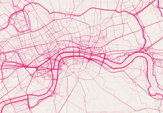

As you can see from the examples above, adjusting the opacity level helped but by adding the multiply blend we can more easily interpret the density of routes.
We can also create some nice effects by using lighter colours on a dark background:


We can also use opacity levels and the multiply blend when we’re mapping terrain. In this example we’re stacking four layers on top of each other (three hillshades and a colour ramp) and tweaking the opacity levels of each. This can help us achieve a much more detail-rich visualisation of the terrain:
As cartographic designers we value the subtleties of map design. It’s important to refine your styles and we highly recommend taking the time to do this. Visualisations, including those above, take a period of trial and error to get right and often very subtle tweaks and techniques can make a big difference – it’s also the fun part!
Let us know if you use these techniques to create your own visualisations.

Our highly accurate geospatial data and printed maps help individuals, governments and companies to understand the world, both in Britain and overseas.